Single capture retrieve
This tutorial shows how to get a full image based on a known outcome_id.
Configuration and imports
Requirements for this demo:
To start, include the packages that we are going to need:
from pystac_client import Client
import geopandas as gpd
import rasterio
import stacmap
import plotly.express as px
import requests
import json
Performing the query and preparing the data
Then, let´s create a connection to the archive API
auth_payload = json.dumps({
  "client_id": "<API_CREDENTIAL_ID>",
  "client_secret": "<API_CREDENTIAL_SECRET>",
  "audience": "https://api.satellogic.com/",
  "grant_type": "client_credentials"
})

auth_headers = {
  'Content-Type': 'application/json'
}

auth_response = requests.request("POST", "https://login.satellogic.com/oauth/token", headers=auth_headers, data=auth_payload)

access_token = auth_response.json()["access_token"]

headers = {"authorizationToken": f"Bearer {access_token}"}

archive = Client.open("https://api.satellogic.com/archive/stac", headers=headers)
Now, we are going to search by outcome id so lets define it:
items = archive.search(
    filter={
        "op": "=",
        "args": [ { "property": "satl:outcome_id" }, outcome_id ]
    },
  ).item_collection()
This query doesn´t need anything else but the outcome_id. By using the item_colletion() method we get all the elements as a pystac object. If they are not needed we can use item_collection_as_dict() to get a Python dict instead.
Analyzing the data
Now, items is a FeatureCollection that contains all the matching items. Items can be accesed with the bracket operator. For example:
We can transform the FeatureCollection into a GeoPandas dataframe for example:
gdf = gpd.GeoDataFrame.from_features(items.to_dict(), crs=f"epsg:{items[0].properties['proj:epsg']}" )
gdf['id'] = [x.id for x in items]
gdf.set_index('id', inplace=True)
gdf['geometry'] = gdf['geometry'].apply(lambda x: x.buffer(0)) # this is because sometimes footprints are not valid polygons, it will be fixed.
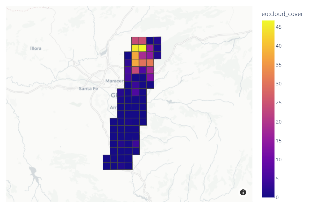
Now we will use this dataframe and plotly to show properties of the data, for example to examine the results in a map and see the cloud cover.
pdf = gdf.reset_index()

# Calculate the centroid of the entire scene to center the map
centroid = pdf.dissolve().centroid[0]

# Plot the entire geometry and use cloud cover as the color for each tile.
fig = px.choropleth_mapbox(
    pdf,
    geojson=pdf.__geo_interface__ ,
    locations=pdf['id'],
    featureidkey='properties.id',
    center={'lat': centroid.y, 'lon':centroid.x},
    zoom=9,
    color="eo:cloud_cover",
    hover_data = ["eo:cloud_cover"]
)

fig.update_layout(
    width=800,
    height=600,
    mapbox_style="carto-positron"
)

fig.show()
This will create an interactive map like this one:

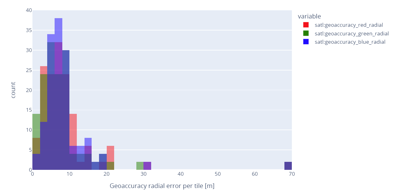
Each of the tiles contains all the metadata fields so we can for example analyze the geolocation error of the set by band with the following code:
fig = px.histogram(
    gdf,
    x=["satl:geoaccuracy_red_radial", "satl:geoaccuracy_green_radial", "satl:geoaccuracy_blue_radial", ],
    color_discrete_sequence=["red", "green", "blue"],
    barmode="overlay",
)

fig.update_layout(
    width=900,
    height=500,
    xaxis_title="Geoaccuracy radial error per tile [m]"
)
fig.show()

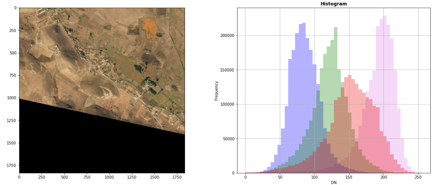
Each tile contains the analytic asset readly availabe. So for exaple using rasterio we can download, show and analyze the image
# Pick one random tile
sample = items[2]

# Load the data
src = rasterio.open(sample.assets['analytic'].href)

# Read the actual bands raster
data = src.read([1,2,3])
display(src.profile)
with rasterio.open('single_tile_example.tif', 'w', **src.profile) as dst:
    dst.write(data.astype(rasterio.uint8), [1,2,3])

# Plot
fig, (axrgb, axhist) = pyplot.subplots(1, 2, figsize=(20,8))
show(data, ax=axrgb)
show_hist(
src, bins=50, lw=0.0, stacked=False, alpha=0.3,
histtype='stepfilled', title="Histogram", ax=axhist)
axhist.get_legend().remove()

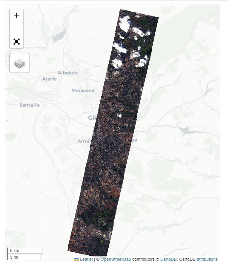
We can also use a tool like stacmap to plot a preview of the entire set on a map:
Previewing the entire set
stacmap.explore(
   items,
   style_kwds={
       "stroke": False,
       "fill": True,
       "fillOpacity": 0,
       },
   #prop="eo:cloud_cover", cmap="BuPu",
   tiles="CartoDB positron",
   fields=["platform", "datetime", "satl:outcome_id", "eo:cloud_cover", "view:sun_elevation", "grid:code"],
   #extensions=["view", "eo"], # or show the entire extension info
   thumbnails=True,
   height=600,
   width = 500
)

From here users can download all the tiles if necessary, and can also create a VRT file with overviews and import it into GIS software like QGIS.